In today’s digital age, the term “neural network” has become synonymous with advancements in artificial intelligence and machine learning. But what exactly are neural networks, and why have they garnered such widespread attention?
What is a Neural Network?
At its core, a neural network is a computational model designed to process information in a way that is reminiscent of how the human brain operates. Just as our brain consists of interconnected neurons that transmit and process information, a neural network is made up of artificial neurons, or “nodes”, that perform similar functions.
| Aspect | Biological Neuron | Artificial Neuron |
|---|---|---|
| Basic Function | Processes and transmits information through electrical and chemical signals. | Receives input, processes it using a mathematical function, and produces an output. |
| Connections | Synapses | Weights and biases |
| Processing Mechanism | Electrochemical processes | Mathematical computations |
| Learning | Changes in synaptic strength | Adjustment of weights and biases based on error |
Why are Neural Networks Important?
Neural networks have the unique ability to “learn” from data. This means that instead of being explicitly programmed to perform a task, they can adjust and adapt based on the information they receive. This adaptability makes them particularly useful for tasks where traditional algorithms struggle, such as image and speech recognition, natural language processing, and even complex game strategies.
Historical Evolution of Neural Networks
The concept of neural networks isn’t a novel invention of the 21st century. In fact, the journey of neural networks traces back several decades, intertwining with the broader history of artificial intelligence and computational neuroscience.
The Dawn of the Idea
The 1940s marked the inception of the neural network concept with the introduction of the McCulloch-Pitts neuron. Warren McCulloch and Walter Pitts proposed a simplified computational model of a biological neuron. This model, though rudimentary, laid the foundation for future developments by demonstrating that a network of artificial neurons could, in theory, compute any logical function.
The Perceptron Era
In 1957, Frank Rosenblatt introduced the Perceptron, a more advanced neural network model. The Perceptron was capable of binary classifications and was one of the earliest models to incorporate learning from its inputs. However, its limitations became evident when it was proven that Perceptrons couldn’t solve non-linearly separable problems, casting doubts on the viability of neural networks.
The AI Winter and the Resurgence
The late 1960s to the early 1980s saw a decline in neural network research, often referred to as the “AI Winter”. This was due to both the limitations of the early models and the rise of alternative AI approaches. However, the 1980s marked a renaissance for neural networks. The introduction of the Backpropagation algorithm by Rumelhart, Hinton, and Williams provided a robust method for training multi-layer networks, paving the way for the development of deep neural networks.
The Anatomy of a Neural Network
Neural networks, in all their complexity, can be broken down into fundamental components that work in tandem to process and learn from data. Let’s dissect these components to understand the intricate machinery that powers these computational marvels.
Layers: The Building Blocks
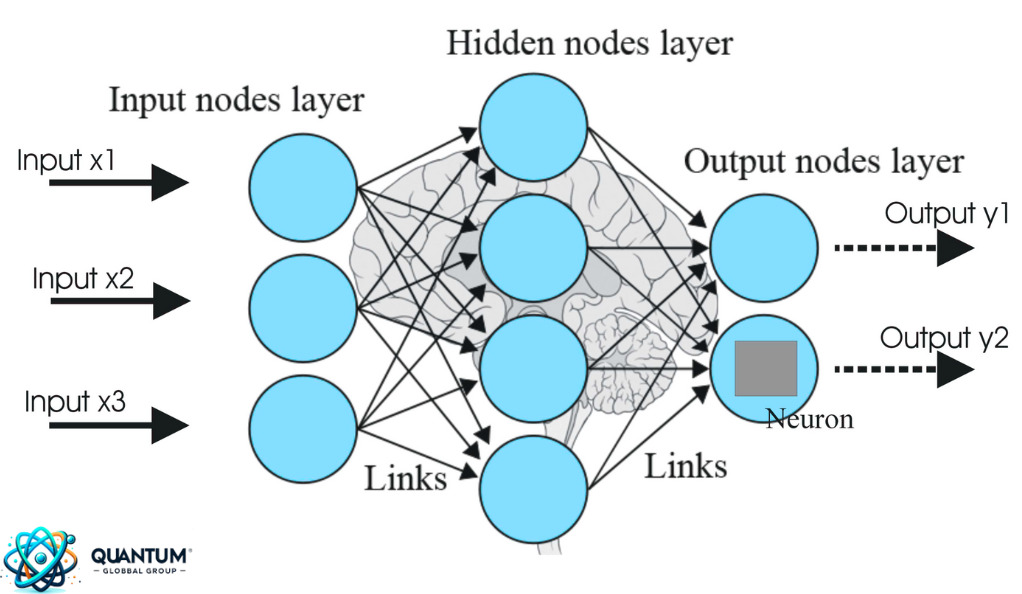
A neural network is typically structured in layers:
- Input Layer: This is the entry point where the network receives data. The number of nodes or neurons in this layer corresponds to the number of input features.
- Hidden Layers: These are sandwiched between the input and output layers. A network can have multiple hidden layers, and this depth is what gives rise to the term “deep learning” in networks with many hidden layers.
- Output Layer: This layer produces the final prediction or classification of the network. The number of neurons here usually corresponds to the number of classes or outputs the network is designed to predict.
Neurons: The Processing Units
Each layer consists of multiple neurons. A neuron receives inputs, multiplies them by weights, adds a bias, and then passes the result through an activation function to produce an output.
| Component | Description |
|---|---|
| Input | Values from the previous layer or external data sources. |
| Weight | A factor that determines the importance of a particular input. Adjusted during the learning process. |
| Bias | A constant added to the weighted sum of inputs to shift the output. |
| Activation Function | Transforms the weighted sum into an output, often introducing non-linearity. Common functions include the sigmoid, ReLU, and tanh. |
Connections: The Pathways of Information
Each neuron in a layer is connected to every neuron in the subsequent layer. These connections have associated weights, which are adjusted during the learning process to minimize the error in predictions.
Learning: The Heart of Neural Networks
The true power of neural networks lies in their ability to learn. Through a process called training, neural networks adjust their weights and biases based on the error of their predictions. The most common method for this is the Backpropagation algorithm, which calculates the gradient of the error and adjusts the weights in the opposite direction to minimize the error.
Learning Paradigms in Neural Networks
The ability of neural networks to adapt and learn from data sets them apart from traditional algorithms. This learning process is governed by various paradigms, each tailored to different types of tasks and data. Let’s delve into these paradigms to understand the mechanisms that drive neural networks’ adaptability.
1. Supervised Learning: Guided Training
In supervised learning, the neural network is trained on a labeled dataset, meaning each input is paired with the correct output. The network makes predictions based on the input, and the error between its predictions and the actual labels is used to adjust its weights and biases.
- Applications:
- Image classification
- Speech recognition
- Predictive analytics
2. Unsupervised Learning: Self-discovery
Unlike supervised learning, unsupervised learning deals with unlabeled data. The network tries to identify patterns or structures within the data without any explicit guidance on what the output should be.
- Applications:
- Clustering (grouping similar data points)
- Dimensionality reduction
- Generative modeling
3. Reinforcement Learning: Learning by Interaction
Reinforcement learning is a dynamic paradigm where the neural network, termed as an agent, interacts with an environment and learns by receiving feedback in the form of rewards or penalties. The goal is to maximize the cumulative reward over time.
- Applications:
- Game playing (e.g., AlphaGo)
- Robot navigation
- Real-time decision-making
4. Semi-supervised and Transfer Learning: Bridging the Gaps
Semi-supervised learning falls between supervised and unsupervised learning. It uses both labeled and unlabeled data, often leveraging small amounts of labeled data to improve learning from a larger pool of unlabeled data.
Transfer learning, on the other hand, involves taking a pre-trained model (trained on a large dataset) and fine-tuning it for a related but different task, thus saving computational resources and time.
- Applications:
- Domain adaptation
- Rapid model deployment with limited data
5. Ensemble Learning: Strength in Numbers
Ensemble methods combine multiple models to produce a single output. The idea is that by leveraging the strengths of multiple models and averaging out their errors, a more robust and accurate prediction can be achieved.
- Applications:
- Random forests
- Boosting algorithms
- Model stacking
Training Neural Networks: The Backpropagation Algorithm
Training is the heartbeat of a neural network. It’s during this phase that a network learns to fine-tune its predictions, adjusting its internal parameters to better fit the data it’s presented with. Central to this process is the Backpropagation algorithm, a method that has stood the test of time and remains pivotal in training deep neural networks.
Understanding the Essence of Backpropagation
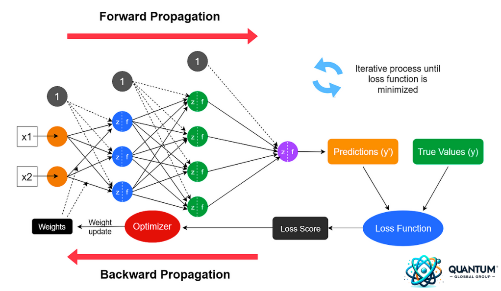
Backpropagation, often abbreviated as “backprop”, is a supervised learning algorithm used for minimizing the error in the predictions of a neural network. The name “backpropagation” stems from the method’s approach: errors are computed at the output and propagated backward through the network’s layers.
The Steps of Backpropagation:
- Forward Pass: Input data is passed through the network, layer by layer, until an output is produced. This is the network’s prediction based on its current weights and biases.
- Compute the Loss: The difference between the network’s prediction and the actual label is calculated using a loss function. Common loss functions include Mean Squared Error for regression tasks and Cross-Entropy for classification.
- Backward Pass: The gradient of the loss with respect to each weight and bias in the network is computed. This is done using the chain rule of calculus, working backward from the output layer to the input.
- Update the Weights and Biases: Using an optimization algorithm, like Gradient Descent or its variants, the weights and biases of the network are adjusted in the direction that reduces the error.
Conclusion
As we journeyed through the intricate world of neural networks, it’s evident that these computational models stand at the forefront of technological innovation. From their biological inspiration to their modern-day applications, neural networks have evolved into powerful tools capable of solving complex problems that were once deemed insurmountable.
Their ability to learn and adapt from data sets them apart, offering a dynamic approach to problem-solving that traditional algorithms couldn’t achieve. Whether it’s recognizing patterns in vast datasets, making predictions, or interacting with dynamic environments, neural networks have showcased unparalleled versatility.

